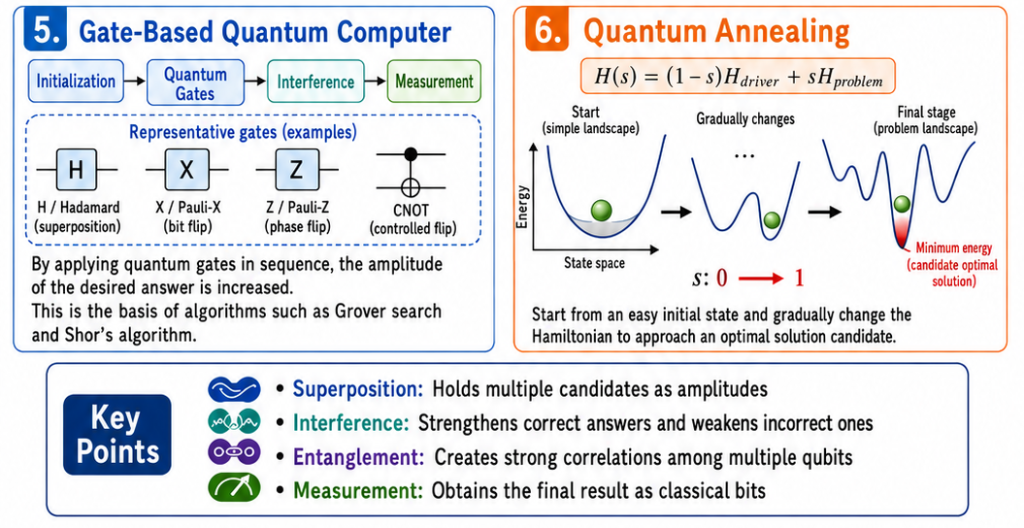
The following code simulates an ideal mathematical model of the inside of a quantum computer using a classical computer.
This code is not “true quantum computation” in the following senses:
・It does not manipulate actual qubits
・It does not utilize quantum hardware
・It does not involve decoherence or gate errors
・It stores the entire amplitude in the memory of a classical computer
・It does not achieve quantum supremacy or quantum acceleration
What This Code Is Calculating
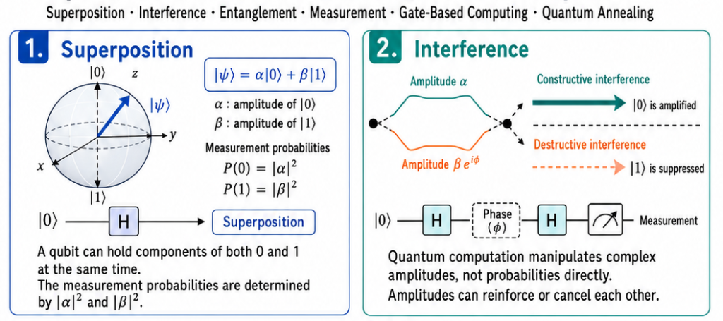
For example, the following array is not a list of classical data. It represents the state vector of a qubit.
ket0 = np.array([1, 0], dtype=complex)This repsents:
The Hadamard gate is also not a statistical operation. It is a unitary matrix representing a quantum gate.
H = (1 / np.sqrt(2)) * np.array([
[1, 1],
[1, -1]
], dtype=complex)
psi = H @ ket0
The result is
which numerically reproduces a qubit in a superposition state.
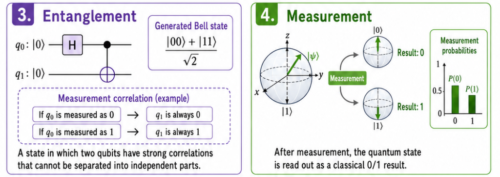
Quantum Entanglement Is Also Reproduced Mathematically
psi = np.kron(ket0, ket0)
psi = np.kron(H, I) @ psi
bell_state = CNOT @ psi
This calculation generates the Bell state. Here, np.kron calculates the tensor product used to construct the combined state of two qubits. This is a quantum-mechanical structure that does not normally appear in ordinary statistical data processing.
"""
An example that simulates representative quantum-computing mechanisms with NumPy.
It can be run in Colab, Jupyter, or a standard Python environment.
"""

import numpy as np
import matplotlib.pyplot as plt

np.set_printoptions(precision=4, suppress=True)

ket0 = np.array([1, 0], dtype=complex)
ket1 = np.array([0, 1], dtype=complex)

I = np.eye(2, dtype=complex)
X = np.array([[0, 1], [1, 0]], dtype=complex)
Z = np.array([[1, 0], [0, -1]], dtype=complex)
H = (1 / np.sqrt(2)) * np.array([[1, 1], [1, -1]], dtype=complex)

CNOT = np.array([
    [1, 0, 0, 0],
    [0, 1, 0, 0],
    [0, 0, 0, 1],
    [0, 0, 1, 0]
], dtype=complex)

basis_1q = ["|0>", "|1>"]
basis_2q = ["|00>", "|01>", "|10>", "|11>"]


def probabilities(state):
    return np.abs(state) ** 2


def measure(state, labels, shots=1000, seed=42):
    rng = np.random.default_rng(seed)
    samples = rng.choice(labels, size=shots, p=probabilities(state))
    unique, counts = np.unique(samples, return_counts=True)
    return dict(zip(unique, counts))


def show_probabilities(state, labels, title):
    probs = probabilities(state)
    print(title)
    for label, prob in zip(labels, probs):
        print(f"  {label}: {prob:.4f}")

    plt.figure(figsize=(6, 3.5))
    plt.bar(labels, probs)
    plt.ylim(0, 1)
    plt.ylabel("Probability")
    plt.title(title)
    plt.show()


def phase_gate(phi):
    return np.array([
        [1, 0],
        [0, np.exp(1j * phi)]
    ], dtype=complex)


def unitary_from_hermitian(hamiltonian, dt):
    eigenvalues, eigenvectors = np.linalg.eigh(hamiltonian)
    return (
        eigenvectors
        @ np.diag(np.exp(-1j * eigenvalues * dt))
        @ eigenvectors.conj().T
    )


# 1. Superposition
superposition = H @ ket0
show_probabilities(
    superposition,
    basis_1q,
    "1. Superposition"
)
print("Measurement:", measure(superposition, basis_1q))


# 2. Interference
phis = np.linspace(0, 2 * np.pi, 200)
p0_values = []
p1_values = []

for phi in phis:
    state = H @ phase_gate(phi) @ H @ ket0
    p0, p1 = probabilities(state)
    p0_values.append(p0)
    p1_values.append(p1)

plt.figure(figsize=(7, 4))
plt.plot(phis, p0_values, label="P(0)")
plt.plot(phis, p1_values, label="P(1)")
plt.xlabel("Phase φ [rad]")
plt.ylabel("Probability")
plt.title("2. Quantum interference")
plt.legend()
plt.grid(True)
plt.show()


# 3. Quantum entanglement
state_00 = np.kron(ket0, ket0)
bell_state = CNOT @ (np.kron(H, I) @ state_00)

show_probabilities(
    bell_state,
    basis_2q,
    "3. Bell-state entanglement"
)
print("Measurement:", measure(bell_state, basis_2q))


# 4. Grover search
uniform_state = np.ones(4, dtype=complex) / 2

oracle = np.eye(4, dtype=complex)
oracle[3, 3] = -1

diffusion = (
    2 * np.outer(uniform_state, uniform_state.conj())
    - np.eye(4, dtype=complex)
)

grover_state = diffusion @ oracle @ uniform_state

show_probabilities(
    grover_state,
    basis_2q,
    "4. Grover search: target |11>"
)


# 5. Quantum annealing
H_driver = -(
    np.kron(X, I)
    + np.kron(I, X)
)
H_problem = -np.kron(Z, Z)

plus = H @ ket0
annealing_state = np.kron(plus, plus)

total_time = 20.0
steps = 1200
dt = total_time / steps

history_s = []
history_ground_probability = []

for step in range(steps):
    s = (step + 0.5) / steps
    H_s = (1 - s) * H_driver + s * H_problem
    annealing_state = (
        unitary_from_hermitian(H_s, dt)
        @ annealing_state
    )

    probs = probabilities(annealing_state)
    history_s.append(s)
    history_ground_probability.append(probs[0] + probs[3])

show_probabilities(
    annealing_state,
    basis_2q,
    "5. Toy quantum annealing"
)

plt.figure(figsize=(7, 4))
plt.plot(history_s, history_ground_probability)
plt.xlabel("Annealing parameter s")
plt.ylabel("P(|00>) + P(|11>)")
plt.ylim(0, 1.02)
plt.title("Ground-state probability")
plt.grid(True)
plt.show()