When you hear the term chaos theory, it sounds like a complex, unmanageable world of mathematics, but in fact it is at work behind the scenes of familiar phenomena and the infrastructure that supports our daily lives.
Chaos theory is a field of study that discovers consistent rules and patterns in complex phenomena that may at first glance appear disjointed. Here are some examples of how it is specifically useful.
1. Weather Forecasting (Ensemble Forecasting)
The most famous concept here is the Butterfly Effect—the idea that a small change (like a butterfly flapping its wings) can cause a massive difference in the outcome (like a tornado). Because weather is a “chaotic system,” it is impossible to predict perfectly. Meteorologists use Ensemble Forecasting, where they run many simulations with slightly different starting points to calculate the probability of rain.
2. Medical Science (Heart Rate Variability)
A healthy human heart does not beat with the perfect regularity of a clock; it has a subtle, chaotic “fluctuation.”
- Heartbeat Analysis: If the heartbeat becomes too predictable or completely random, it often signals health issues like heart failure.
- Brain Waves: Our brain activity is also chaotic. Doctors study these patterns to predict seizures in patients with epilepsy.
3. Communication & Cryptography
Chaos theory generates sequences that look like random noise but are actually based on specific mathematical rules.
- Chaos Encryption: This is used to hide data. To an outsider, the message looks like “static” or “noise,” but the receiver with the correct “key” (the mathematical formula) can decode it perfectly.
4. Financial Markets
The stock market is a classic complex system. While it is nearly impossible to predict the exact price of a stock tomorrow, chaos theory helps analysts understand the “volatility” (instability) of the market to manage financial risks.
5. Home Appliances (Chaos Control)
In Japan, you might have seen products advertised with “fluctuations”
- Washing Machines & Fans: Some high-end fans use chaos theory to simulate a “natural breeze.” Because a constant wind speed feels unnatural to the human body, these devices vary the airflow in a chaotic yet rhythmic way to make it more comfortable.
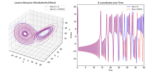
The Lorenz Attractor (The Butterfly Effect)
This script visualizes how a tiny difference in starting conditions leads to completely different outcomes.
import numpy as np
import matplotlib.pyplot as plt
from scipy.integrate import odeint
from mpl_toolkits.mplot3d import Axes3D

# Define the Lorenz equations
def lorenz(state, t, sigma, rho, beta):
    x, y, z = state
    dxdt = sigma * (y - x)
    dydt = x * (rho - z) - y
    dzdt = x * y - beta * z
    return [dxdt, dydt, dzdt]

# Parameters
sigma = 10.0
rho = 28.0
beta = 8.0 / 3.0
t = np.arange(0.0, 40.0, 0.01)

# Two starting points with a tiny difference (0.00001) in the z-axis
state1 = [1.0, 1.0, 1.0]
state2 = [1.0, 1.0, 1.00001]

# Solve the differential equations
data1 = odeint(lorenz, state1, t, args=(sigma, rho, beta))
data2 = odeint(lorenz, state2, t, args=(sigma, rho, beta))

# Plotting
fig = plt.figure(figsize=(12, 6))

# Left: 3D Visualization
ax1 = fig.add_subplot(1, 2, 1, projection='3d')
ax1.plot(data1[:, 0], data1[:, 1], data1[:, 2], color='blue', alpha=0.7, lw=0.5, label='Start: 1.0')
ax1.plot(data2[:, 0], data2[:, 1], data2[:, 2], color='red', alpha=0.5, lw=0.5, label='Start: 1.00001')
ax1.set_title("Lorenz Attractor (Butterfly Effect)")
ax1.set_xlabel("X axis")
ax1.set_ylabel("Y axis")
ax1.set_zlabel("Z axis")
ax1.legend()

# Right: Time Series Comparison (X-coordinate)
ax2 = fig.add_subplot(1, 2, 2)
ax2.plot(t, data1[:, 0], color='blue', label='Start: 1.0', alpha=0.7)
ax2.plot(t, data2[:, 0], color='red', linestyle='--', label='Start: 1.00001', alpha=0.7)
ax2.set_title("Divergence of X-coordinate Over Time")
ax2.set_xlabel("Time")
ax2.set_ylabel("X Value")
ax2.legend()

plt.tight_layout()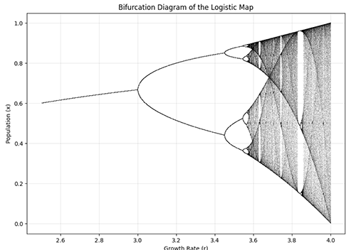
plt.show()The Logistic Map (Bifurcation Diagram)
This script shows the transition from a stable system to a chaotic one using a simple iterative formula.
import numpy as np
import matplotlib.pyplot as plt

def logistic_map():
    # Settings
    n = 10000          # Number of values for growth rate (r)
    iterations = 1000  # Total iterations to reach stability
    last = 100         # Number of points to plot for each r

    # Range for r (Growth rate from 2.5 to 4.0)
    r = np.linspace(2.5, 4.0, n)
    # Initial population x
    x = 1e-5 * np.ones(n)

    plt.figure(figsize=(10, 7))

    # Calculation and plotting
    for i in range(iterations):
        # The Logistic Map formula: x = r * x * (1 - x)
        x = r * x * (1 - x)

        # After many iterations, plot the last few results
        if i >= (iterations - last):
            # ',k' means pixel-sized black dots
            plt.plot(r, x, ',k', alpha=0.1)

    plt.title("Bifurcation Diagram of the Logistic Map")
    plt.xlabel("Growth Rate (r)")
    plt.ylabel("Population (x)")
    plt.grid(True, alpha=0.3)
    plt.show()

if __name__ == "__main__":
    logistic_map()